240P/NEAT

240P/NEAT
Originally uploaded by cbellh47

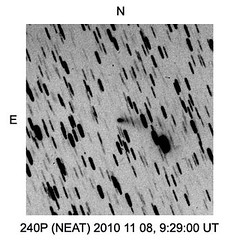
Comet 240P/NEAT on morning of November 8, 2010 with long curved dust tail.

Discovery of Comet Hartley 2 - 1986 Apparition

Comet Hartley 2 was discovered on March 15, 1986 by Malcolm Hartley at the U. K. Schmidt Telescope Unit, Siding Spring Observatory, New South Wales. The comet was initially designated as 1986c in IAUC 4197.

Discovery image of comet 103P?Hartley
at 1986 03 15.59361
Anglo-Australian Observatory (AAO) with the UK Schmidt Telescope

The comet showed up as a diffuse streak on a photographic plate taken on March 15, 1986. M. Hartley made additional observations were made on March 17, and March 20, 1986. These three observations are given in IAUC 4197 and a preliminary parabolic orbit computed (e =1 assumed) . The initial calculated perihelion date of T = 1985 June 20.07 ET, showed that the comet was seven months post-perihelion and outbound from earth and sun. Earth distance = 3.476 AU. Solar Distance r = 4.452 AU putting the comet between the orbit of Mars and Jupiter. The initial magnitude was 17.5 T or "Total comet magnitude".

Subsequent observations in April 1986 by Oak Ridge Observatory and Palomar Observatory were submitted and the orbit refined confirming that the comet was had an elliptical orbit, e < 1, and was periodic with a short period (P < 200 years). 

Perihelion Date T = 1985 June 5.053 ET

Perihelion distance q = 0.96099 AU

eccentricty e =  0.71563

inclination i =  9.181 degrees

Period 6.21 years

Peri. = 174.670 

Node = 226.609 

semi-major axis a = 3.37933 AU 

Daily orbital motion n = 0.158657 degrees/day

The 1986 computed orbit shows that comet 103P/Hartley passed close to Jupiter on November 1982 and again in December 1993

Kazuo Kinoshita Comet Orbit Page for 103P shows close approach to Jupiter:

Jupiter  0.3255 AU on 19821102.5

Jupiter  0.3743 AU on 19931219.3

----------------------

MPC observatory code 413
Code Long.        cos          sin               Name
413 149.06608 0.855595 -0.516262  Siding Spring Observatory

The UK Schmidt Telescope (UKST) has an aperture of 1.2 metres and a very wide-angle field of view. The telescope was commissioned in 1973. The telescope was designed to photograph 6.6 x 6.6 degree areas of the night sky on plates 356 x 356 mm (14 x 14 inches) square.






------------------
Using MPCOBS on the Minor Planet Center web site
1986 observations of comet 103P:

0103PJ86E020  A1986 03 15.59361 11 25 25.15 -07 44 15.6          17.5 T 10592413
0103PJ86E020  A1986 03 17.67951 11 23 26.88 -07 27 42.7                 10592413
0103PJ86E020  A1986 03 20.60691 11 20 45.41 -07 04 21.9                 10592413
0103PJ86E020  A1986 04 04.12772 11 09 13.39 -05 11 29.2                 10592801
0103PJ86E020  A1986 04 05.16007 11 08 32.84 -05 03 52.1                 10592801
0103PJ86E020  A1986 04 05.20583 11 08 30.96 -05 03 31.3          18   T 10592675
0103PJ86E020  A1986 04 05.21069 11 08 30.75 -05 03 28.7                 10592675
0103PJ86E020  A1986 04 05.21750 11 08 30.50 -05 03 26.0                 10592675
0103PJ86E020  A1986 04 08.15569 11 06 41.19 -04 42 22.9                 10592675
0103PJ86E020  A1986 04 08.16097 11 06 40.99 -04 42 20.5                 10592675
0103PJ86E020  A1986 04 08.17083 11 06 40.64 -04 42 16.4                 10592675
0103PJ86E020  A1986 05 10.15791 10 58 11.07 -01 59 12.5                 10794691
0103PJ86E020  A1986 05 10.17935 10 58 11.11 -01 59 08.3                 10794691
0103PJ86E020  A1986 05 10.19726 10 58 11.16 -01 59 04.9                 10794691
0103PJ86E020  A1986 05 12.08925 10 58 17.95 -01 53 34.6                 10794801
0103PJ86E020  A1986 06 07.15793 11 05 31.14 -01 23 08.0                 10892691
0103PJ86E020  A1986 06 07.16865 11 05 31.41 -01 23 08.9                 10892691
0103PJ86E020  A1986 06 07.22340 11 05 32.86 -01 23 09.9                 10892691

------------------------------------------
IAUC 4197 1986 March 24

COMET HARTLEY (1986c)

     Malcolm Hartley, U.K. Schmidt Telescope Unit, Siding Spring,
reports his discovery of a comet of magnitude ~ 17-18 with a faint
tail evident:

           1986 UT             R.A.   (1950.0)   Decl.

           Mar. 15.59361     11 22 52.78     - 7 27 45.7
                17.67951     11 20 54.53     - 7 11 14.2
                20.60691     11 18 13.08     - 6 47 55.4

     The following parabolic orbital elements are very uncertain.
A low-inclination, short-period orbit gives similar residuals.

         T = 1985 June 20.07 ET  Peri. = 185.39
                                 Node  = 179.23   1950.0
         q =   0.0759 AU         Incl. =  59.76

     1986 ET     R.A. (1950.0) Decl.      p        r       m1

     Mar. 11    11 27.33    - 8 04.2    3.476    4.452    17.2
          21    11 17.86    - 6 44.8
          31    11 09.42    - 5 27.2    3.733    4.678    17.6
     Apr. 10    11 02.34    - 4 15.0
          20    10 56.79    - 3 11.1    4.118    4.898    18.0
          30    10 52.84    - 2 17.0
     May  10    10 50.41    - 1 33.4    4.594    5.114    18.4
          20    10 49.40    - 1 00.2
          30    10 49.65    - 0 36.8    5.120    5.325    18.8

1986 March 24                  (4197)            Daniel W. E. Green

-------------------------

IAUC 4200: 1986c;

PERIODIC COMET HARTLEY 2 (1986c)
     The following precise positions have been reported:

    1986 UT           R.A.   (1950.0)  Decl.    m1   Observer

    Apr.  5.16007   11 06 00.40   - 4 47 36.4        Schwartz
          5.20583   11 05 58.52   - 4 47 15.6   18   Gibson
          5.21069   11 05 58.31   - 4 47 13.0          "
          5.21750   11 05 58.06   - 4 47 10.3          "

G. Schwartz (Oak Ridge Observatory).  1.5-m reflector.  Weak image.
   Measurer: C.-Y. Shao.
J. Gibson (Palomar Observatory).  1.5-m reflector + CCD.

     A computation from the observations Mar. 15-Apr. 5 confirms
this to be a short-period comet (cf. IAUC 4197).  The solar elongation
would have been too small to permit observations near perihelion.
The revolution period is somewhat uncertain, but the
comet evidently made a rather close approach to Jupiter in 1982.

          T = 1985 June 5.053 ET
      Peri. = 174.670                    e =   0.71563
      Node  = 226.609   1950.0           a =   3.37933 AU
      Incl. =   9.181                    n =   0.158657
          q =   0.96099 AU               P =   6.21 years

     1986 ET     R.A. (1950.0) Decl.      p        r       m1

     Mar. 31    11 09.61    - 5 26.2    2.362    3.312    17.6
     Apr. 10    11 03.09    - 4 13.4
          20    10 58.59    - 3 10.7    2.641    3.446    18.0
          30    10 56.16    - 2 20.6
     May  10    10 55.68    - 1 43.8    3.001    3.575    18.4
          20    10 56.98    - 1 20.1
          30    10 59.81    - 1 08.7    3.407    3.699    18.8
     June  9    11 03.96    - 1 08.3
          19    11 09.21    - 1 17.7    3.825    3.818    19.2
          29    11 15.36    - 1 35.7
     July  9    11 22.25    - 2 01.1    4.230    3.932    19.6

1986 April 8                   (4200)              Brian G. Marsden

-------------------------

Comet 103P/Hartley 2 (1986c) on November 2, 1982 near Jupiter

Comet 103P/Hartley 2 (1986c) on June 5, 1985 at perihelion.
Comet elongation low 

Comet 103P/Hartley 2 (1986c) on March 15, 1986 at discovery.
Comet near earth opposition. 

Comet 103P/Hartley 2 (1986c) on December 19, 1993 near Jupiter

References:

UK Schmidt Telescope (UKST): http://www.aao.gov.au/ukst/
IAUC 4197: http://www.cfa.harvard.edu/iauc/04100/04197.html
IAUC 4200: http://www.cfa.harvard.edu/iauc/04200/04200.html
Seiichi Yoshida Comet Page: http://www.aerith.net/comet/catalog/0103P/index.html

Kazuo Kinoshita Comet Orbit Home Page: http://jcometobs.web.fc2.com/pcmtn/0103p.htm

Cometary Orbit Viewer: http://www.astroarts.com/simulation/cometary-orbit.php
CDS Image Server discovery image of comet 103P from the "Second Epoch Survey" of the southern sky was made by the Anglo-Australian Observatory (AAO) with the UK Schmidt Telescope digitized and compressed by the SScI: http://aladin.u-strasbg.fr/java/alapre-ok.pl?-c=11+25+25.15+-07+44+15.6&out=image&fmt=FITS&resolution=FULL&qual=SERC+ER+DSS2

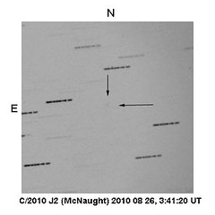
Comet C/2010 J2 (McNaught)

Comet C/2010 J2 (McNaught)
Originally uploaded by cbellh47

Comet C/2010 J2 (McNaught)
18 x 151 sec
0.3-m f/4.7 Schmidt-Cassegrain + CCD + red filter
Time Stamp: 2010 08 26, 3:41:20 UT
Motion: 1.03"/min in PA 276.2°
Diffuse. Weakly condensed coma
Magnitude: 18.2 N

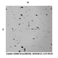
Comet C/2006 S3 (LONEOS)

Comet C/2006 S3 (LONEOS)
Originally uploaded by cbellh47

Comet C/2006 S3 (LONEOS)
4x272s
0.3-m f/4.7 Schmidt-Cassegrain + CCD + Red Filter
Time Stamp: 2010 08 27, 4:41:18 UT
Motion: 0.60"/min in PA 251.1°
Mag 17.0 N

JAXA Hayabusa-2 mission planned to asteroid (162173) 1999 JU3

Japan Aerospace Exploration Agency (JAXA) Hayabusa-2 mission to asteroid 162173 (1999 JU3)  is in the planning stage. The plan is to launch Hayabusa-2 in 2014, land on the asteroid in 2018 and gather surface samples and return to Earth in 2020. The return trip of 2 years versus 6 year total mission time).  The Hayabusa-2  probe will use explosives to make a hole on the asteroid to collect surface materials. JAXA recently announced it submitted a proposal to the country's Space Activities Commission for a less ambitious follow-on to Hayabusa costing about $310 million. The commission and Japanese government will decide the fate of Hayabusa 2 when the JAXA budget is formulated later this year. On Wednesday the trial production of equipment to be loaded on the Hayabusa-2 space probe was approved.

JAXA image

Hayabusa-2 Spacecraft

• ion propulsion
• almost same as first Hayabusa with minor modifications
• flat antenna
• approach involves one Earth swingby
• Minerva 2 - Lander
• sample collection from the asteroid surface with "touch-and-go" approach

Hayabusa-2 and Minerva 2 - Lander (JAXA image)

Orbital diagram of NEA 162173 

(162173) 1999 JU3

• C-type asteroid
• SMASSII spectral class Cg
• expected to contain more organic or hydrated materials than S-type Itokawa
• a = 1.1896212 AU
• e = 0.1902258
• P = 1.30 years
• Apollo or earth crossing Near Earth Asteroid (NEA)
• Potentially Hazard Asteroid  (PHA)
• Discovered 1999-May-10 by LINEAR at Socorro (704)
 

Kyodo News: http://home.kyodo.co.jp/modules/fstStory/index.php?storyid=516945

The Daily Yomiuri - Panel OK's development of Hayabusa successor: http://www.yomiuri.co.jp/dy/features/science/T100805005346.htm

Spaceflight Now - ESA's Cosmic Vision missions depend on priorities abroad: 

http://www.spaceflightnow.com/news/n1007/23cosmicvision/

Hayabusa-2 -http://www.jspec.jaxa.jp/e/activity/hayabusa2.html#

Asteroid explorer Hayabusa-2  http://b612.jspec.jaxa.jp/mission/e/hayabusa2_e.html

Astrometry 101 - How long of exposure can my image frames be?

There is no hard and fast rule other than long enough to get  reasonable SNR on reference stars and your target. Sets of images can be can be easily aligned (process called image registration) and stacked in a number of ways such as add, median combine, averaging. The goal of astrometry is position measurement, not photometry. With photometry, the higher the SNR, the better the result, with 50 highly desired. But such SNRs are not so practical for faint objects. For astrometry, the SNR of the target should be at least 5. You should be able to detect movement of the target with at least two observations to ensure the target is not a star, if performing comet or asteroid astrometry.

A general rule of thumb for exposure length is the time it takes for the moving object to move one pixel.

To determine this you need to know how fast an object is moving across the sky.

pixel scale  = (206.265) * (pixel size in microns) / (focal length in mm)

If your pixel scale is 2.5 arc sec/pixel and your target is moving at 0.01 arc sec/sec, then you can expose for up to (2.5 arc sec/pixel) / (0.01 arc sec/sec) or 250 seconds for one pixel movement.

Depending on light pollution in your area, your images may be background limited. Light pollution causes the same effect  in your images as you see as the sun comes up in the morning, the sky brightens and stars fade and lose SNR. Bright moonlight causes the same stellar extinction phenomenon as the sky background dominates the stellar light signal ad they disappear.

The large aperture survey telescopes may only expose for 30 seconds in order to reach a certain magnitude desired such as magnitude 21. A smaller aperture scope such as a 0.3 meter or 12 inch scope will be limited by the sky or object movement and pixel scale.

To go for fainter comets and asteroids, you can do a number of things:

• use a focal reducer to get closer to optimal pixel scale.
• stack images
• bin camera pixels to increase effective pixel size
• get a larger aperture scope 

To find how fast an object is moving across the sky, sky motion, you can use a number of resources.

Minor Planet and Comet Ephemeris Service: http://www.cfa.harvard.edu/iau/MPEph/MPEph.html

You can select to display motions as:  "/sec   "/min   "/hr   °/day

You can also select to separate R.A. and Decl. sky motions instead of total sky motion to squeeze a little more exposure time depending on whether RA (or x) or Decl. (or y) is more limiting.

A planetarium program such as TheSky6Pro displays sky motion in the info dialog of solar system bodies including the sun, moon, planets, comets, and minor planets.

JPL has an ephemeris service or HORIZONS Web-Interface: http://ssd.jpl.nasa.gov/horizons.cgi

Generally the closer to earth or sun an object is, the faster its sky motion and brightness.

A faint target can also be moving more quickly and you may need a larger image stack or shorter exposures.

Observing known comets and asteroids makes this decision process easier to predict and plan.

There is the possibility that a new or unknown object may show up in your images, with main belt asteroids being the most likely. By using an average sky motion for these objects, you can limit your exposure times based on that, so that an object will not produce a long streak in an image, but a measurable centroid. The larger aperture scopes have a distinct advantage over smaller scopes here because of their immense light gathering power not limited by object motion but by how deep or faint they want to survey. The general idea is to gather three or more images (or sets of images if stacking)  separated by 10 to 15 minutes each so that any moving objects will readily show up when blinking images or when using software detection. Distant objects such as Pluto, Centaurs, Kuiper Belt Objects (KBOs), or TransNeptunian objects (TNOs) may require time separation of an hour or more to detect them. Large aperture survey telescopes have the advantage of stopping down their focal length and flattening the image field so as to image larger portions of the sky and more efficiently survey the sky.

Reference:

IAU Minor Planet Center Guide to Minor Body Astrometry:

http://www.cfa.harvard.edu//iau/info/Astrometry.html

Astrometry 101 - Pixel Scale

Every astrometry observer and measurer needs to know the pixel scale of their images. This is the angular width and height of a pixel. Pixel scale tells how much of the sky is covered by one pixel.  Many CCD cameras have square pixels (equal height and width). If the camera pixels are not square, then both dimensions musts be considered. Normally width is denoted by x and height y.

To calculate pixel scale, one needs telescope focal length and pixel width or height in microns.

pixel scale or sampling in arcseconds = (206.265) * (pixel size in microns) / (focal length in mm)

or

focal length = (206.265) * (pixel size in microns) /  pixel scale

The constant 206.265 converts microns to mm and radians to arc seconds.

A micrometer or micron is one millionth of a meter, or equivalently one thousandth of a millimeter (mm)

[360 deg / (2 pi radians)] x (3600 arc sec / deg) x ( 1 mm / 1000 microns) = 206.26480624709635515647335733078 ~= 206.265

or just about 206 as many use as rule of thumb.

This is a straightforward calculation if you know the two input parameters.

Focal ratio is the ratio of the focal length to telescope aperture

Focal ratio = focal length / aperture

For example, if focal length = 3048 mm and  aperture = 30.48 mm, Focal ratio = 10 or telescope is at f /10.
If you have 9 micron square CCD pixels, then your pixel scale is  206.265 x 9 / 3048  or 0.6 arc sec per pixel.

This has meaning when compared to your "seeing" measured in arc secs of FHWM (Full Width Half Maximum) of the stars in your images and is referred to as "sampling". You have near optimal sampling when your pixel scale is about half of the value of your seeing. If your pixel scale is less than optimal, the sampling is termed "under sampled". If your pixel scale is larger than optimal, the sampling is termed "over sampled".

Focal reducers reduce the effective focal length of your imaging setup and increase your pixel scale.
Binning your CCD camera imaging chip 2x2 (versus high resolution 1x1) doubles the size of each pixel and increases your pixel scale.

Barlow lenses increase the effective focal length of your imaging setup and decrease your pixel scale.

Astrometrica calculates these parameters for you if you can interpret the values provided after doing a plate solution. The default values of its configuration settings must be initially modified by a new user for their imaging setup. Thus, one must be able to calculate or estimate a focal length as an input parameter for this program.

This is  a copy of several lines in a recent Astrometrica.log file from my own astrometry:

The column labeled FHWM reports the seeing of the stars in the image and shows that sthe seeing is about 5 to 6 arc seconds. The pixel size is calculated at 2.58 arc sec or about half the seeing. I was using 2x2 binning on a SBIG ST-8XME CCD camera. There is a f/6.3 focal reducer a filter wheel and an SBIG AO-7 unit in the imaging setup, but due to the spacing of the components resulting in an effective focal ratio of near 4.7. This also gives a nice size field of view to capture more stars which is better for accurate astrometry. The SNR of the stars measured for astrometry is also given. It is important to have sufficient SNR for an accurate centroid calculation of stars and the object to be measured. The Fit RMS is the most important columns because it shows the bottom line of the astrometric calculation and the goal is to have fractional arc second accuracy is all measurements..

Pixel scale is used to determine how long of an exposure one can take of a moving object. That will be the subject of another topic.

The larger your pixel scale the longer you can expose your target per image.

The larger your pixel scale, you provide allow more photons from your target to fall on a pixel which improves the SNR of your target, improves the calculation of the target centroid in the image, improves astrometric precision, and results in smaller residuals.(only up to optimal)

Too high a pixel scale beyond optimal however, is not good for astrometry because stars will be undersampled and are not spread out over one or more pixels. It would be like trying to accurately measure the position of a fly with a ruler with only inch or centimeter tick marks. and is of no astrometric value no matter how reference stars you have imaged..

Reference:

IAU Minor Planet Center Guide to Minor Body Astrometry:

http://www.cfa.harvard.edu//iau/info/Astrometry.html